The previous module explored how price affects the quantity demanded and the quantity supplied. The result was the demand curve and the supply curve. Price, however, is not the only factor that influences demand, nor is it the only thing that influences supply. For example, how is demand for vegetarian food affected if health concerns cause more consumers to avoid eating meat? How is the supply of diamonds affected if diamond producers discover several new diamond mines? What are the major factors, in addition to the price, that influence demand or supply?

When economists talk about supply, they mean the amount of some good or service a producer is willing to supply at each price. Price is what the producer receives for selling one unit of a good or service. A rise in price almost always leads to an increase in the quantity supplied of that good or service, while a fall in price will decrease the quantity supplied. When the price of gasoline rises, for example, it encourages profit-seeking firms to take several actions: expand exploration for oil reserves; drill for more oil; invest in more pipelines and oil tankers to bring the oil to plants for refining into gasoline; build new oil refineries; purchase additional pipelines and trucks to ship the gasoline to gas stations; and open more gas stations or keep existing gas stations open longer hours. Economists call this positive relationship between price and quantity supplied—that a higher price leads to a higher quantity supplied and a lower price leads to a lower quantity supplied—the law of supply. The law of supply assumes that all other variables that affect supply (to be explained in the next module) are held constant.

Still unsure about the different types of supply? See the following Clear It Up feature.

CLEAR IT UP

Is supply the same as quantity supplied?

In economic terminology, supply is not the same as quantity supplied. When economists refer to supply, they mean the relationship between a range of prices and the quantities supplied at those prices—a relationship that we can illustrate with a supply curve or a supply schedule. When economists refer to quantity supplied, they mean only a certain point on the supply curve, or one quantity on the supply schedule. In short, supply refers to the curve and quantity supplied refers to the (specific) point on the curve.

Figure 2.8 illustrates the law of supply, again using the market for gasoline as an example. Like demand, we can illustrate supply using a table or a graph. A supply schedule is a table, like Table 2.3, that shows the quantity supplied at a range of different prices. In Table 2.3 we measure price in dollars per gallon of gasoline and we measure quantity supplied in millions of gallons. A supply curve is a graphic illustration of the relationship between price, shown on the vertical axis, and quantity, shown on the horizontal axis. The supply schedule and the supply curve are just two different ways of showing the same information. Notice that the horizontal and vertical axes on the graph for the supply curve are the same as for the demand curve.

Table 2.3 Price and Supply of Gasoline

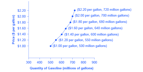
Price (per gallon)	Quantity Supplied (millions of gallons)
$1.00	500
$1.20	550
$1.40	600
$1.60	640
$1.80	680
$2.00	700
$2.20	720

The shape of supply curves will vary somewhat according to the product: steeper, flatter, straighter, or curved. Nearly all supply curves, however, share a basic similarity: they slope up from left to right and illustrate the law of supply: as the price rises, say from $1.00 per gallon to $2.20 per gallon, the quantity supplied increases from 500 gallons to 720 gallons. Conversely, as the price falls, the quantity supplied decreases.

How Production Costs Affect Supply

A supply curve shows how quantity supplied will change as the price rises and falls, assuming ceteris paribus so that no other economically relevant factors are changing. If other factors relevant to supply do change, then the entire supply curve will shift. Just as we described a shift in demand as a change in the quantity demanded at every price, a shift in supply means a change in the quantity supplied at every price.

In thinking about the factors that affect supply, remember the firms’ motivations: profits, specifically the difference between revenues and costs. A firm produces goods and services using combinations of labor, materials, and machinery, or what we call inputs or factors of production. If a firm faces lower costs of production, while the prices for the good or service remain unchanged, their profits go up. When a firm’s profits increase, it is more motivated to produce output, since the more it produces the more profit it will earn. When costs of production fall, a firm will tend to supply a larger quantity at any given price for its output. We can show this by the supply curve shifting to the right.

Take, for example, a messenger company that delivers packages around a city. The company may find that buying gasoline is one of its main costs. If the price of gasoline falls, then the company will find it can deliver messages more cheaply than before. Since lower costs correspond to higher profits, the messenger company may now supply more of its services at any given price. For example, given the lower gasoline prices, the company can now serve a greater area, and increase its supply.

Conversely, if a firm faces higher costs of production, then it will earn lower profits at any given selling price for its products. As a result, a higher cost of production typically causes a firm to supply a smaller quantity at any given price. In this case, the supply curve shifts to the left.

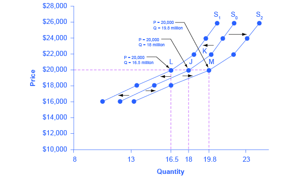
Consider the supply of cars, shown by curve (S₀) in Figure 2.9. Point (J) indicates that if the price is $20,000, the quantity supplied will be 18 million cars. If the price rises to $22,000 per car, in situations of ceteris paribus the quantity supplied will rise to 20 million cars, as point (K) on curve (S₀) shows. We can show the same information in table form, as in Table 2.4.

Now, imagine that the price of steel, an important ingredient in manufacturing cars, rises, so that producing a car has become more expensive. At any given price for selling cars, car manufacturers will react by supplying a lower quantity. We can show this graphically as a leftward shift of supply, from S₀ to S₁, which indicates that at any given price, the quantity supplied decreases. In this example, at a price of $20,000, the quantity supplied decreases from 18 million on the original supply curve (S₀) to 16.5 million on the supply curve (S₁), which is labeled as point (L).

Conversely, if the price of steel decreases, producing a car becomes less expensive. At any given price for selling cars, car manufacturers can now expect to earn higher profits, so they will supply a higher quantity. The shift of supply to the right, from S₀ to S₂, means that at all prices, the quantity supplied has increased. In this example, at a price of $20,000, the quantity supplied increases from 18 million on the original supply curve (S₀) to 19.8 million on the supply curve (S₂), which is labeled M.

Other Factors That Affect Supply

In the example above, we saw that changes in the prices of inputs in the production process will affect the cost of production and thus the supply. Several other things affect the cost of production, too, such as changes in weather or other natural conditions, new technologies for production, and some government policies.

Changes in weather and climate will affect the cost of production for many agricultural products. For example, in 2014, Northeastern China’s Manchurian Plain (which produces most of the country’s wheat, corn, and soybeans) experienced its most severe drought in over 50 years. A drought decreases the supply of agricultural products, which means that at any given price, a lower quantity will be supplied. Conversely, especially good weather would shift the supply curve to the right.

When a firm discovers a new technology that allows them to produce at a lower cost, the supply curve will shift to the right. For instance, in the 1960s a major scientific effort nicknamed the Green Revolution focused on breeding improved seeds for basic crops like wheat and rice. By the early 1990s, more than two-thirds of the wheat and rice in low-income countries around the world used Green Revolution seeds—and the harvest was twice as high per acre. A technological improvement that reduces costs of production will shift supply to the right, so that a greater quantity is produced at any given price.

Government policies can affect the cost of production and the supply curve through taxes, regulations, and subsidies. For example, the U.S. government imposes a tax on alcoholic beverages that collects about $8 billion per year from producers. Firms treat taxes as costs. Higher costs decrease supply for the reasons we discussed above. Other examples of policy that can affect cost are the wide array of government regulations that require firms to spend money to provide a cleaner environment or a safer workplace. Complying with regulations increases costs.

A government subsidy, on the other hand, is the opposite of a tax. A subsidy occurs when the government pays a firm directly or reduces the firm’s taxes if the firm carries out certain actions. From the firm’s perspective, taxes or regulations are an additional cost of production that shifts supply to the left, leading the firm to produce a lower quantity at every given price. Government subsidies reduce the cost of production and increase supply at every given price, shifting supply to the right. The following Work It Out feature shows how this shift happens.

WORK IT OUT

Shift in Supply

We know that a supply curve shows the minimum price a firm will accept to produce a given quantity of output. What happens to the supply curve when the cost of production goes up? The following is an example of a shift in supply due to a production cost increase.

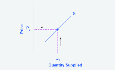
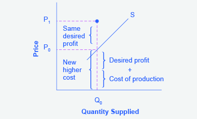
Step 1. Draw a graph of a supply curve for pizza. Pick a quantity (like Q0). If you draw a vertical line up from Q0 to the supply curve, you will see the price the firm chooses. Figure 2.10 provides an example.

 

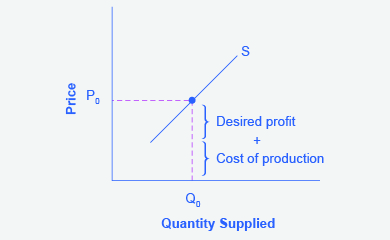
Step 2. Why did the firm choose that price and not some other? One way to think about this is that the price is composed of two parts. The first part is the cost of producing pizzas near the margin; in this case, the cost of producing the pizza, including cost of ingredients (e.g. dough, sauce, cheese, and pepperoni), the cost of the pizza oven, the shop rent, and the workers’ wages. The second part is the firm’s desired profit, which is determined, among other factors, by the profit margins in that particular business (desired profit is not necessarily the same as economic profit, which will be explained in Chapter 7). If you add these two parts together, you get the price the firm wishes to charge. The quantity Q0 and associated price P0 give you one point on the firm’s supply curve, as Figure 2.11 illustrates.

 

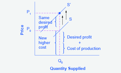
Step 3. Now, suppose that the cost of production increases. Perhaps cheese has become more expensive by $0.75 per pizza. If that is true, the firm will want to raise its price by the amount of the increase in cost ($0.75). Draw this point on the supply curve directly above the initial point on the curve, but $0.75 higher, as Figure 2.12 shows.

 

Step 4. Shift the supply curve through this point. You will see that an increase in cost causes an upward (or a leftward) shift of the supply curve so that at any price, the quantities supplied will be smaller, as Figure 2.13 illustrates.

 

Summing Up Factors That Change Supply

Cost of production is affected by changes in the cost of inputs, natural disasters, new technologies, and the impact of government decisions. In turn, these factors affect how much firms are willing to supply at any given price.

Figure 2.14 summarizes factors that change the supply of goods and services. Notice that a change in the price of the product itself is not among the factors that shift the supply curve. Although a change in price of a good or service typically causes a change in quantity supplied or a movement along the supply curve for that specific good or service, it does not cause the supply curve itself to shift.

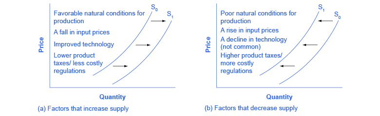
Because demand and supply curves appear on a two-dimensional diagram with only price and quantity on the axes, an unwary visitor to the land of economics might be fooled into believing that economics is about only four topics: demand, supply, price, and quantity. However, demand and supply are really “umbrella” concepts: demand covers all the factors that affect demand, and supply covers all the factors that affect supply. Factors other than price that affect demand and supply are illustrated by using shifts in the demand and supply curve. In this way, the two-dimensional demand and supply model becomes a powerful tool for analyzing a wide range of economic circumstances.