Equilibrium—Where Demand and Supply Intersect

Because the graphs for demand and supply curves both have price on the vertical axis and quantity on the horizontal axis, the demand curve and supply curve for a particular good or service can appear on the same graph. Together, demand and supply determine the price and the quantity that will be bought and sold in a market.

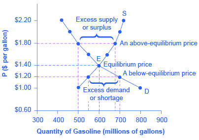
Figure 2.15 illustrates the interaction of demand and supply in the market for gasoline. The demand curve (D) is identical to Figure 2.2. The supply curve (S) is identical to Figure 2.8. Table 2.4 contains the same information in tabular form.

Table 2.4 Price, Quantity Demanded, and Quantity Supplied

Remember this: When two lines on a diagram cross, this intersection usually means something. The point where the supply curve (S) and the demand curve (D) cross, designated by point (E) in Figure 2.15, is called the equilibrium. The equilibrium price is the only price where the plans of consumers and the plans of producers agree—that is, where the amount of the product consumers want to buy (quantity demanded) is equal to the amount producers want to sell (quantity supplied). Economists call this common quantity the equilibrium quantity. At any other price, the quantity demanded does not equal the quantity supplied, so the market is not in equilibrium at that price.

In Figure 2.15, the equilibrium price is $1.40 per gallon of gasoline and the equilibrium quantity is 600 million gallons. If you had only the demand and supply schedules, and not the graph, you could find the equilibrium by looking for the price level on the tables where the quantity demanded and the quantity supplied are equal.

The word “equilibrium” means “balance.” If a market is at its equilibrium price and quantity, then it has no reason to move away from that point. However, if a market is not at equilibrium, then economic pressures arise to move the market toward the equilibrium price and the equilibrium quantity. Imagine, for example, that the price of a gallon of gasoline was above the equilibrium price—that is, instead of $1.40 per gallon, the price is $1.80 per gallon. The dashed horizontal line at the price of $1.80 in Figure 2.15 illustrates this above-equilibrium price. At this higher price, the quantity demanded drops from 600 to 500. This decline in quantity reflects how consumers react to the higher price by finding ways to use less gasoline. Moreover, at this higher price of $1.80, the quantity of gasoline supplied rises from the 600 to 680, as the higher price makes it more profitable for gasoline producers to expand their output. Now, consider how quantity demanded and quantity supplied are related at this above-equilibrium price. Quantity demanded has fallen to 500 gallons, while quantity supplied has risen to 680 gallons. In fact, at any above-equilibrium price, the quantity supplied exceeds the quantity demanded. We call this an excess supply or a surplus.

With a surplus, gasoline accumulates at gas stations, in tanker trucks, in pipelines, and at oil refineries. This accumulation puts pressure on gasoline sellers. If a surplus remains unsold, those firms involved in making and selling gasoline are not receiving enough cash to pay their workers and to cover their expenses. In this situation, some producers and sellers will want to cut prices, because it is better to sell at a lower price than not to sell at all. Once some sellers start cutting prices, others will follow to avoid losing sales. These price reductions in turn will stimulate a higher quantity demanded. Therefore, if the price is above the equilibrium level, incentives built into the structure of demand and supply will create pressures for the price to fall toward the equilibrium.

Now suppose that the price is below its equilibrium level at $1.20 per gallon, as the dashed horizontal line at this price in Figure 2.15 shows. At this lower price, the quantity demanded increases from 600 to 700 as drivers take longer trips, spend more minutes warming up the car in the driveway in wintertime, stop sharing rides to work, and buy larger cars that get fewer miles to the gallon. However, the below-equilibrium price reduces gasoline producers’ incentives to produce and sell gasoline, and the quantity supplied falls from 600 to 550.

When the price is below equilibrium, there is excess demand, or a shortage—that is, at the given price the quantity demanded, which has been stimulated by the lower price, now exceeds the quantity supplied, which had been depressed by the lower price. In this situation, eager gasoline buyers mob the gas stations, only to find many stations running short of fuel. Oil companies and gas stations recognize that they have an opportunity to make higher profits by selling what gasoline they have at a higher price. As a result, the price rises toward the equilibrium level. Read the section Consumer Surplus, Producer Surplus, and Deadweight Loss for more discussion on the importance of the demand and supply model.